Nodebox demos

This is a selection of demos from Nodebox 1, by the Nodebox authors (Frederik de Bleser and Tom de Smedt), with slight edits.

Math sculpture

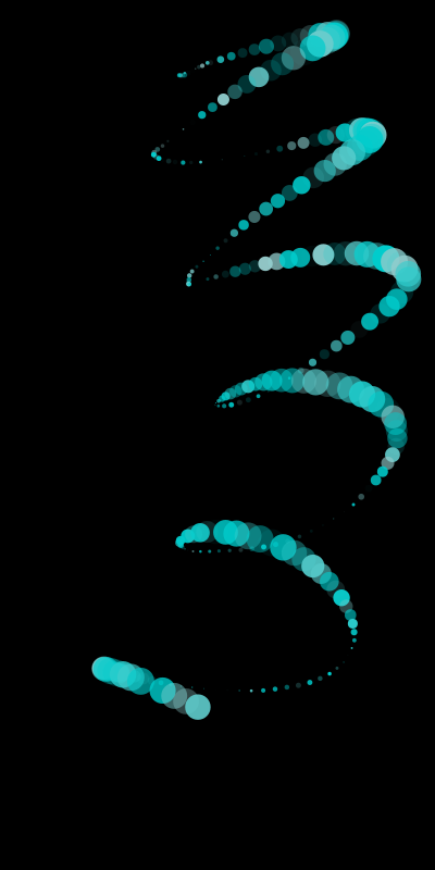
Generates sculptures using a set of mathematical functions. Every iteration adds a certain value to the current coordinates. Rewriting this program to use transforms is left as an exercise for the reader.

from math import sin, cos, log10

size(400, 800)
background(0)

cX = random(1, 10)
cY = random(1, 10)

x = 200
y = 54
fontsize(10)

for i in range(278):
    x += cos(cY) * 11
    y += log10(cX) * 1.85 + sin(cX) * 5

    fill(random() - 0.4, 0.8, 0.8, random())

    s = 10 + cos(cX) * 15
    oval(x - s / 2, y - s / 2, s, s)
    # Try the next line instead of the previous one to see how
    # you can use other primitives.
    # star(x-s/2, y-s/2, random(5, 10), inner=2+s*0.1, outer=10+s*0.1)

    cX += random(0.25)
    cY += random(0.25)

Color grid

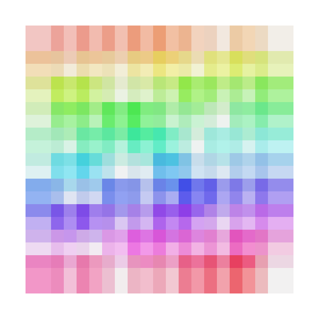
This example showcases the HSB color mode to select colors more naturally, by specifying a hue, saturation and brightness.

size(625, 625)

colormode(HSB)

# Set some initial values. You can and should play around with these.
h = 0
s = 0.5
b = 0.9
a = 0.5

# Size is the size of one grid square.
square_size = 50

# Using the translate command, we can give the grid some margin.
translate(50, 50)

# Create a grid with 10 rows and 10 columns. The width of the columns
# and the height of the rows is defined in the 'size' variable.
for x, y in grid(10, 10, square_size, square_size):
    # Increase the hue while choosing a random saturation.
    # Try experimenting here, like decreasing the brightness while
    # changing the alpha value etc.
    h += 0.01
    s = random()

    # Set this to be the current fill color.
    fill(h, s, b, a)

    # Draw a rectangle that is one and a half times larger than the
    # grid size to get an overlap.
    rect(x, y, square_size * 1.5, square_size * 1.5)

Ball grid

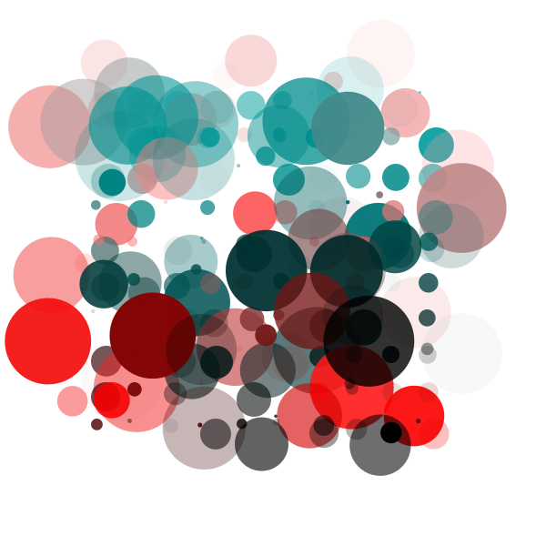
Use a grid to generate a bubble-like composition.

This example shows that a grid doesn’t have to be rigid at all. It’s very easy to break loose from the coordinates Shoebot passes you, as is shown here. The trick is to add or subtract something from the x and y values Shoebot passes on. Here, we also use random sizes.

from math import sin, cos

size(600, 600)

gridSize = 40

# Translate a bit to the right and a bit to the bottom to
# create a margin.
translate(100, 100)

startval = random()
c = random()
for x, y in grid(10, 10, gridSize, gridSize):
    fill(sin(startval + y * x / 100.0), cos(c), cos(c), random())
    s = random() * gridSize
    oval(x, y, s, s)
    fill(cos(startval + y * x / 100.0), cos(c), cos(c), random())
    deltaX = (random() - 0.5) * 10
    deltaY = (random() - 0.5) * 10
    deltaS = (random() - 0.5) * 200
    oval(x + deltaX, y + deltaY, deltaS, deltaS)
    c += 0.01

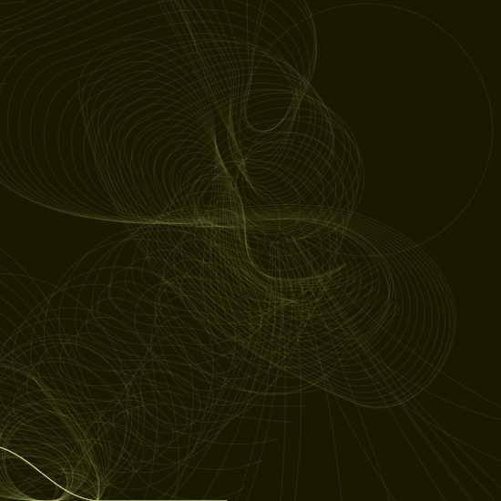
Blines and circloids

by Tom de Smedt <https://www.nodebox.net/code/index.php/Blines_and_Circloids>

# You'll need the Boids and Cornu libraries.
boids = ximport("boids")
cornu = ximport("cornu")

size(550, 550)
background(0.1, 0.1, 0.0)
nofill()

flock = boids.flock(10, 0, 0, WIDTH, HEIGHT)

n = 70
for i in range(n):

    flock.update(shuffled=False)

    # Each flying boid is a point.
    points = []
    for boid in flock:
        points.append((boid.x, boid.y))

    # Relativise points for Cornu.
    for i in range(len(points)):
        x, y = points[i]
        x /= 1.0 * WIDTH
        y /= 1.0 * HEIGHT
        points[i] = (x, y)

    t = float(i) / n
    stroke(0.9, 0.9, 4 * t, 0.6 * t)
    cornu.drawpath(points, tweaks=0)

Color grid

This example showcases the HSB color mode to select colors more naturally, by specifying a hue, saturation and brightness.

size(625, 625)

colormode(HSB)

# Set some initial values. You can and should play around with these.
h = 0
s = 0.5
b = 0.9
a = 0.5

# Size is the size of one grid square.
square_size = 50

# Using the translate command, we can give the grid some margin.
translate(50, 50)

# Create a grid with 10 rows and 10 columns. The width of the columns
# and the height of the rows is defined in the 'size' variable.
for x, y in grid(10, 10, square_size, square_size):
    # Increase the hue while choosing a random saturation.
    # Try experimenting here, like decreasing the brightness while
    # changing the alpha value etc.
    h += 0.01
    s = random()

    # Set this to be the current fill color.
    fill(h, s, b, a)

    # Draw a rectangle that is one and a half times larger than the
    # grid size to get an overlap.
    rect(x, y, square_size * 1.5, square_size * 1.5)

Circles and Beziers

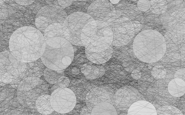
size(640, 400)
colorrange(255)
colormode(HSB)
background(0, 0, 192)

for i in range(0, WIDTH // 4, 1):
    # ^ range requires a float, so use integer division '//'
    sz = random(WIDTH / 40, WIDTH / 5)
    xpos = random(-WIDTH / 5, WIDTH)
    ypos = random(-WIDTH / 5, HEIGHT)

    fill(0, 0, random(192, 224), random(85, 255))
    ellipse(xpos, ypos, sz, sz)

    nofill()
    stroke(0, 0, 0, 255)
    strokewidth(.1)
    ellipse(xpos, ypos, sz, sz)

    for j in range(0, WIDTH // 80, 1):
        # ^ range requires a float, so use integer division '//'
        stroke(0, 0, 0, 255)
        strokewidth(.1)
        beginpath(random(-WIDTH / 2, WIDTH * 1.5), random(-HEIGHT / 2, HEIGHT * 1.5))
        curveto(random(-WIDTH / 2, WIDTH * 1.5), random(-HEIGHT / 2, HEIGHT * 1.5),
                random(-WIDTH / 2, WIDTH * 1.5), random(-HEIGHT / 2, HEIGHT * 1.5),
                random(-WIDTH / 2, WIDTH * 1.5), random(-HEIGHT / 2, HEIGHT * 1.5))
        endpath()